I’m an engineer working where applied AI, data science and operations research meet.
I hold an engineering degree from Arts et Métiers (France) and a research master’s (MSc.A) from Polytechnique Montréal, where my thesis on AI for tender response was completed.
I build tools that turn messy, real-world data into decisions: LLM agents, retrieval pipelines, ranking models and optimization methods. I like to understand every layer of what I build.
Projects
Selected projects
Applied AI & agents
In guarding and patrol services almost every contract is won through a public call
for tenders, yet bids were priced by intuition while available data could improve the response
process. For my research MSc thesis at Polytechnique Montréal, with a
leading Québec security-services company, I designed, built and evaluated an
end-to-end decision-support tool: it finds the tender, reads its
100–200-page specification, retrieves comparable past contracts and recommends the
highest margin that still wins.
01 — How it works
Five modules around one shared database
Every module reads from or writes to a single store covering January 2015 to
March 2026. The modules are chained, so an extraction error propagates into the
recommended price; each one is therefore validated on its own.
01
Monitor
Scrape the Québec tendering system (SEAO) and link each new tender to its past versions with entity resolution, so renewals are spotted before they are announced.
02
Read
Hierarchical RAG and a local LLM turn the specification PDF into structured requirements (uniforms, equipment, vehicles), then into dollar scores.
03
Compare
A similarity score whose weights are re-adjusted from rankings made by bid experts.
04
Price
Rank a grid of candidate margins instead of regressing one, so the model optimises what the business cares about.
05
Show
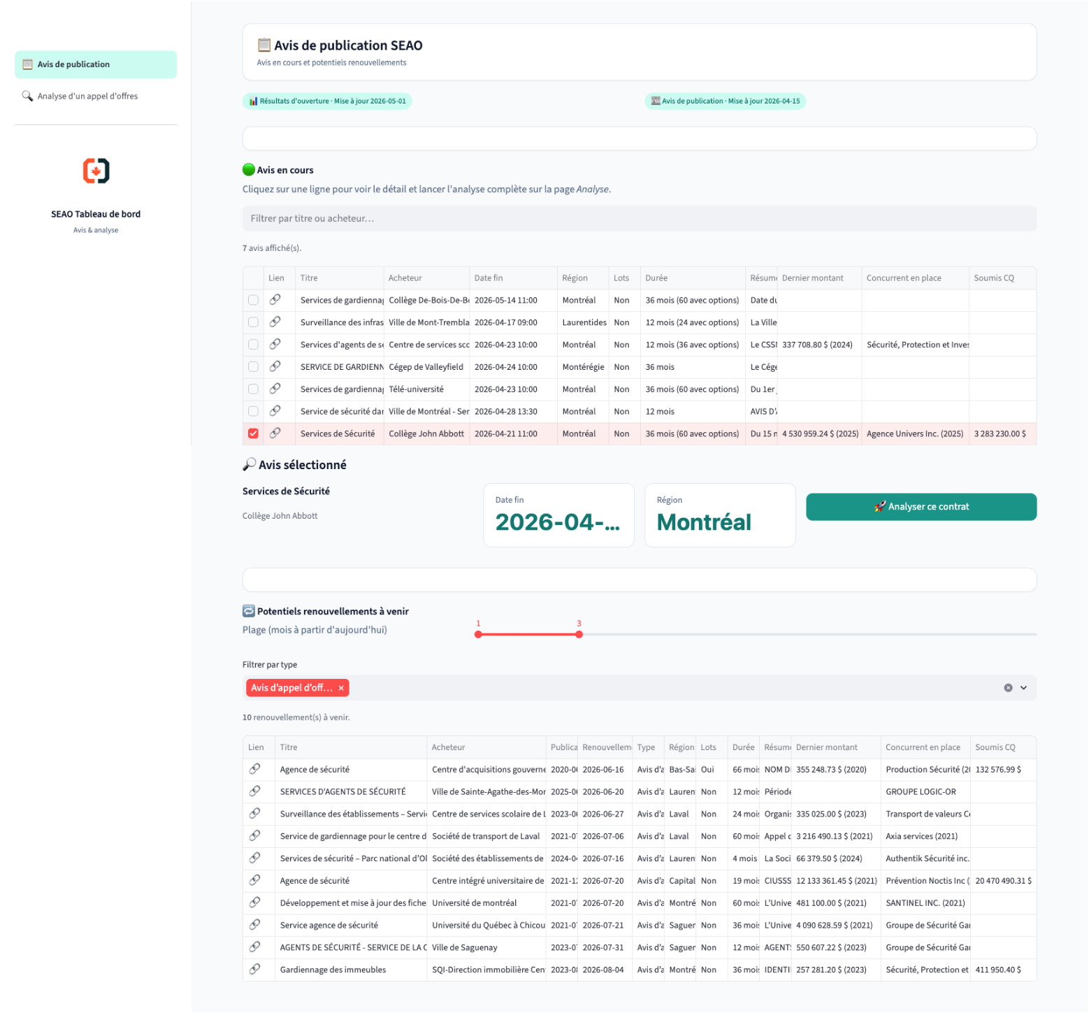
A Streamlit app for bid managers: opportunities, contract analysis, competitor profiles and the recommended margin.
The extraction pipeline (module 2). The document structure is kept when chunking, retrieval is sparse and domain-specific, and the LLM answers into a fixed JSON schema; a cost dictionary then turns the text into comparable numbers.
02 — Skills
LLM and RAG. Hierarchical retrieval over contract PDFs: PyMuPDF layout
parsing, section-aware chunking, BM25 with a security-domain vocabulary, and
schema-constrained JSON extraction by a local quantised LLM
(Ministral-3-14B), so confidential documents never leave the company.
Learning from human feedback. A small neural network retrained with a RankNet
pairwise loss on expert rankings to learn what "comparable contract" means.
Learning to Rank. Pricing reframed as ranking candidate margins with
XGBRanker (pairwise objective, NDCG), which fits the asymmetric business loss and
small data better than regression.
NLP and entity resolution. spaCy matching against a cost dictionary;
Levenshtein and SequenceMatcher to link contracts written differently every time.
Data engineering and deployment. Selenium scraping, one shared database,
Streamlit, Docker on Azure (ADLS Gen2).
Applied research. Design Research Methodology, process redesign in BPMN with
the partner's bid managers, leak-free chronological evaluation.
03 — Results
87% precision / 98% recall for the RAG extraction, on 50 labelled contracts.
92% concordance when linking 60 tenders of 2025 to their past contracts.
40% win rate against 15% for the company's own pricing, and
+10% projected profits, in chronological
leave-one-out on 54 tenders.
On a second run of 57 tenders, ranked first on 59% and in the
top three on 83%.
Same win rate, twice the money. Regression wins as often as the ranking model, but minimising error pushes every bid down; ranking keeps the margin.
Monitoring. Ongoing tenders and upcoming renewals; one click opens the analysis.
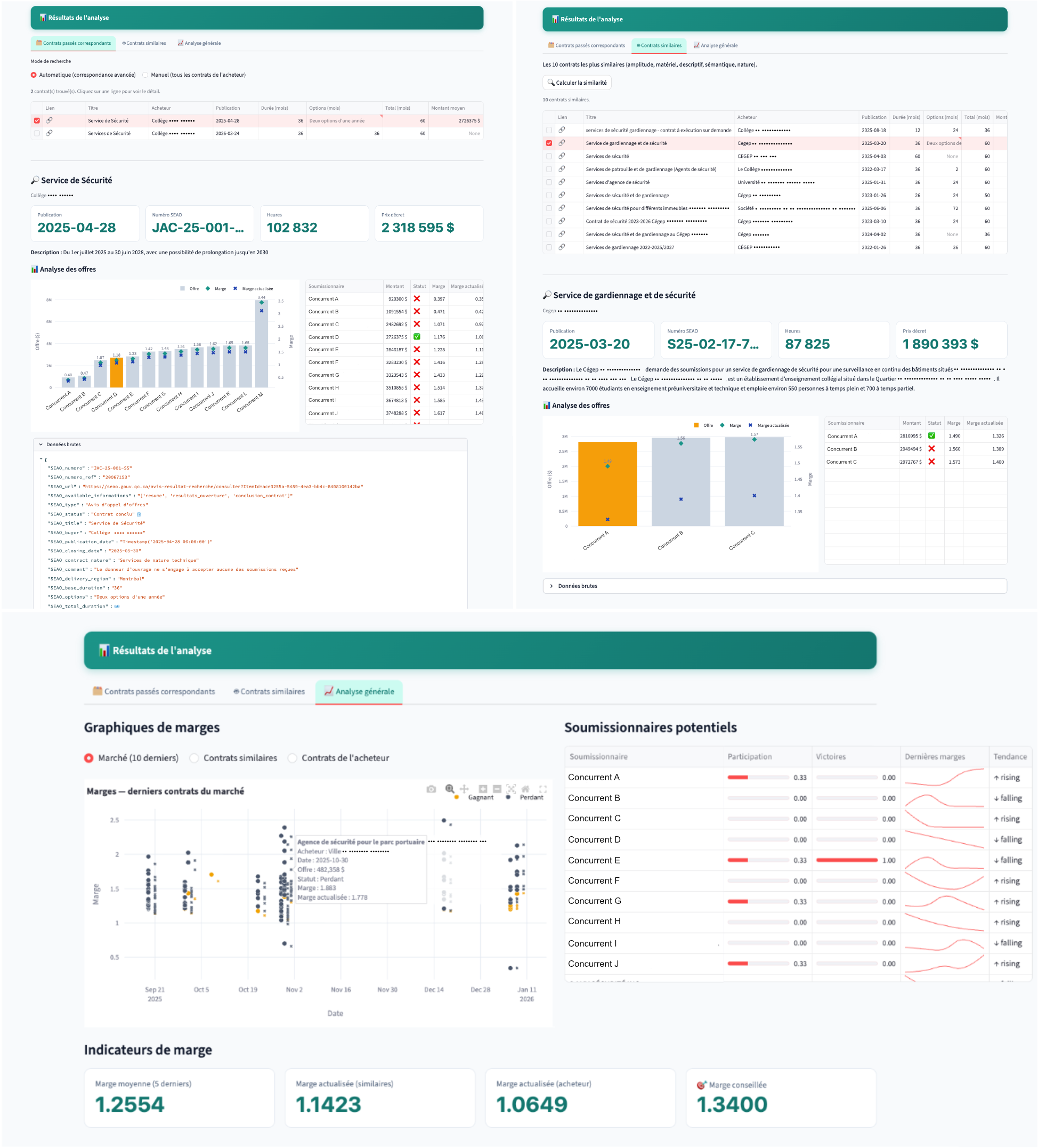
Contract analysis. Past versions, similar contracts and the market view that ends on a recommended margin.
Conference paper (accepted): E. Salaun, M. Belmouadden, R. Pellerin, A. Neumann,
C. Vasseur, "Leveraging artificial intelligence and strategic data for tender response
processes", CENTERIS 2026. Polytechnique
Montréal and CIRRELT, with Commissionnaires du Québec; funded by Mitacs. Results are
retrospective, and every recommendation is reviewed by an expert. The contract data is
confidential; the rest of the work is published in a public thesis; figures are redrawn
for this page.
"Which buildings around Saint Joseph's Oratory are taller than 20 m?" Answering that
from airborne LiDAR takes a chain of GIS and machine-learning steps on 127 million
points. This project puts an LLM agent in front of that chain with one rule:
the LLM plans and explains, it never computes. Every number comes
from a deterministic tool, and a validator checks each result before the LLM sees
it.
01 — How it works
Three nodes, seven tools, one validator
The agent is a LangGraph state machine. The agent node is a single
Claude API call that picks the next tool; tools runs typed Python
functions; validator applies physical and geometric rules (no LLM) and
sends errors back with likely causes and a suggested fix, with at most two retries.
Tools exchange file paths, so every intermediate result is cached and can be opened in
QGIS: a follow-up question reuses the earlier files instead of starting over.
The tools, in the order of the standard plan.
Tool
Returns
find_lidar_tiles
tile extents and density
load_point_cloud
the requested area, cropped from the tiles
normalize_height
height above ground and a terrain model
classify_lidar_points
a class for every point
extract_buildings
footprints with heights and areas (GeoJSON)
filter_buildings
buildings within a height range
create_map
an interactive map
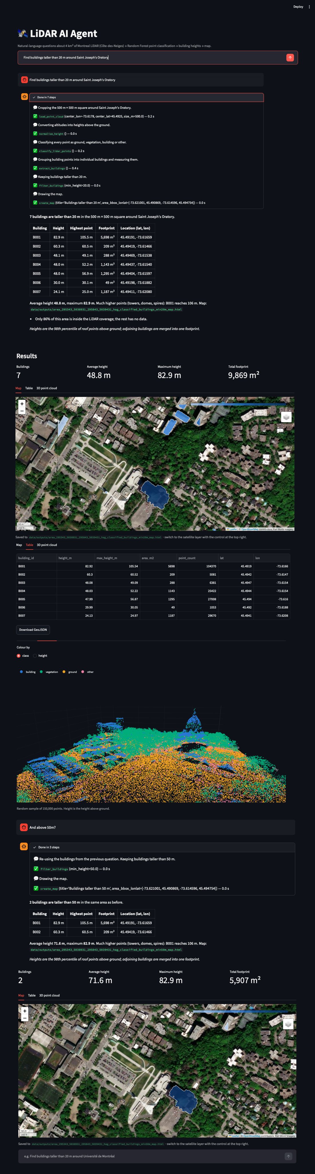
A question and its follow-up (scroll inside the frame), with the live trace of every tool call. The follow-up takes 3 steps instead of 7 because it reuses the first answer's buildings file.
02 — Skills
LLM agents and tool use. Claude function calling orchestrated by LangGraph;
an 80-line decorator turns type hints into JSON schemas and validates arguments with
pydantic.
Guardrails. A rule-based validator between the tools and the LLM, which
checks every building in a result and not only the ones the LLM sees, plus an offline
planner when no API key is available.
Machine learning on 3D data. A Random Forest point classifier with
geometric features (linearity, planarity, scattering, verticality) from local
covariance; spatially held-out evaluation, so test points never neighbour training
points.
GIS. Terrain normalisation, raster morphology and vectorised footprints
with GeoPandas and rasterio; Folium maps and a 3D view in Streamlit.
Testing LLM systems. 25 tests run without an API key: scripted fake LLMs
drive the real graph, tools and validator.
03 — Results
0.914 building F1 (0.880 without the geometric features), 0.929 accuracy,
on 480,000 held-out points.
Buildings found from the predicted classes against the vendor's professional
classification: 36 / 36 matched, 0.04 m median height difference,
footprint IoU 0.944.
About 35 s from raw tiles to a map for a 500 m × 500 m area, on a laptop.
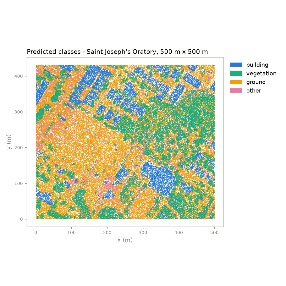
Predicted classes around the Oratory. Roofs, canopy and open
ground come out as coherent patches.
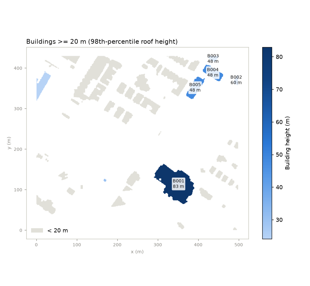
Buildings of at least 20 m around the Oratory. The basilica (B001)
has an 83 m roof height and a highest point at 106 m.
Personal project. Known limits: adjoining buildings merge into one
footprint, vegetation training labels are derived by rule, and the validator's 150 m
limit must be raised for downtown Montreal.
Québec publishes every public tender, bid and award as open data, but as
multi-gigabyte nested JSON that cannot answer a simple question. This project turns that
feed into a query-ready SQLite database and exposes it to Claude or ChatGPT through a
read-only MCP server. The point is not to
give the model SQL access, which a generic server already does, but to give it
the correct SQL, built into tools, for the questions where the
obvious query returns a plausible but wrong number.
01 — How it works
Three build scripts, one server, nine tools
Three idempotent scripts download, filter and normalise the feed into 18 tables
and 5 views, with an accent-insensitive full-text index and a data dictionary stored
in the database itself. A FastMCP server then offers six curated analytical tools for
the questions worth getting right, and three flexible ones
(describe_schema, search_processes, run_sql)
for everything else.
Nine tools, one door. Every question goes either to a curated tool or to the flexible core, through the same read-only connection.
Three traps that a model writing its own SQL falls into, and that the tools handle for it.
Trap
What goes wrong
How the tools handle it
Supplier identity
One firm, many spellings: Garda alone is 9 legal entities under 6 names
Names are resolved to all their enterprise numbers before aggregating
Win and loss
Not stored; counting bid rows double-counts lots
Derived from award membership, counted per tender
Direct awards
No bids at all, so a firm handed 3 contracts scores 100%
Excluded from win rates, always reported alongside
02 — Skills
Tool design for LLMs (MCP). Tools designed backwards from analysts'
questions; they return short reports in the analyst's vocabulary rather than raw
rows, and the server's handshake instructions give the model the data rules before
its first call.
LLM guardrails.run_sql is read-only by construction rather
than by instruction: a read-only database connection, a single SELECT statement
with a blocklist of write commands, a 2,000-row cap and a 5-second timeout.
Data modelling. Nested Open Contracting (OCDS) releases normalised into
a relational schema, with entity resolution of suppliers.
Data engineering. An incremental download, a filter that can be retargeted
to another sector in two lists, a normaliser using only the standard library.
03 — Results
A plain-language question such as "Garda's win rate on open tenders?" becomes one
tool call. The server works in Claude Code and Claude Desktop, and in ChatGPT through
a proxy. A smoke test calls all nine tools with the README's example questions,
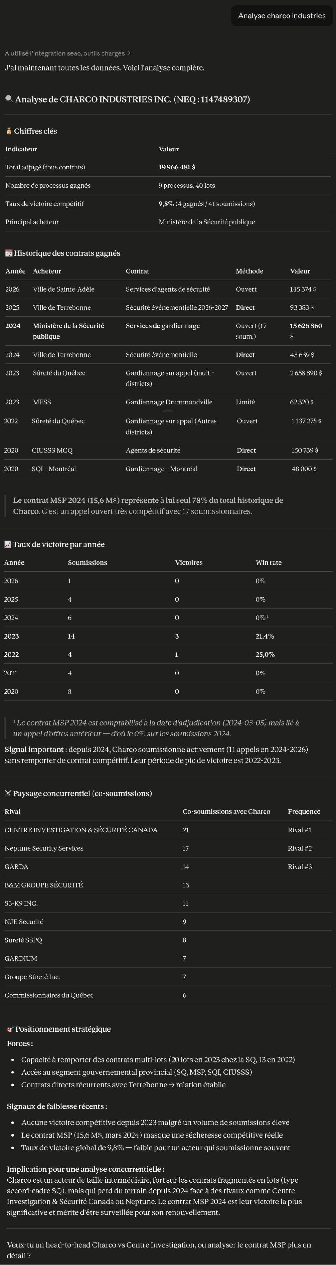
including a DELETE that has to be refused. Below, a three-word prompt
produces a full competitor analysis in which every number comes from a tool call.
"Analyse charco industries" (scroll inside the frame): key figures, contract history, win rate by year and most frequent rivals, then Claude's reading of them.
Open-source tool, MIT licence. Data: Québec SEAO open data (OCDS) via
open.canada.ca, security services only; coverage skews to 2021–2025, so figures are
indicative.
Can a 9-billion-parameter model running locally (Qwen 3.5 9B in LM
Studio, on a MacBook Air) play a real-time strategy game well? Not by looking at
328,000 map tiles. This agent reduces OpenFront
to a graph, gives the model a short situation text and a menu of
legal options, and splits it into two roles: a strategist that plans and
a commander that gives orders. The code enforces the plan between calls.
01 — How it works
The LLM chooses what, the code chooses where
The unmodified OpenFront engine runs headless in the same process, and game time
pauses while the model thinks. Each change becomes a sentence ("Queensland started
attacking you with 46,040 troops"). The strategist, called every 20 s or on major
events, gets the core rules plus the 6 most relevant of 37 knowledge sections and
writes a plan: priorities, a focus, the troop reserve to keep and the size of expansion
waves. The commander, called only when something changes, turns it into at most two
orders as JSON. The schema is rebuilt every turn and its enum is the current list of
legal option ids, so an invalid order cannot be written.
// a real commander turn from the winning match, at 3:15
{
  "reason": "Carolinian Republic eliminated; attack Carolinian
             Commonwealth to secure west, then build city for
             growth. Keep 35% reserve (682,942 troops) ...",
  "actions": [
    { "id": "attack_carolinian_commonwealth", "troops_percent": 30 },
    { "id": "build_city", "troops_percent": 0 }
  ]
}
02 — Skills
LLM agent design. A planner/executor split, event-driven calls, and a
self-check that sends a rule-breaking answer back once with the numbers.
Structured output. A JSON schema whose enum is the menu of legal options,
with maxLength on every text field so an answer can never be cut off
mid-JSON.
Retrieval without embeddings. 37 tagged knowledge sections; the situation
picks 6, deterministically, and every factual section is checked against the real
engine by a test.
State abstraction. 328,000 tiles → a graph of ~30 players (borders, attacks,
alliances) → a short text a 9B model can reason about.
Integrating a large codebase. The OpenFront engine at a pinned commit,
fetched with a sparse checkout (7 MB instead of 1.3 GB).
Evaluation and reproducibility. Scripted baselines on the same seed, offline
reproductions of failures without the LLM, every prompt and answer logged to
turns.jsonl, and 39 Vitest tests, including a full match with a mock LLM
that runs a 30-minute game in seconds.
03 — Results
On the Australia map against 7 AI nations and 20 tribes (Easy, seed
australia-1), the LLM won outright after 8 min 49 s with 80.9% of
the land, ranked first from the first minute. 130 LLM calls (29 strategist,
101 commander), 0 errors, 8.0 s mean latency, no cloud API.
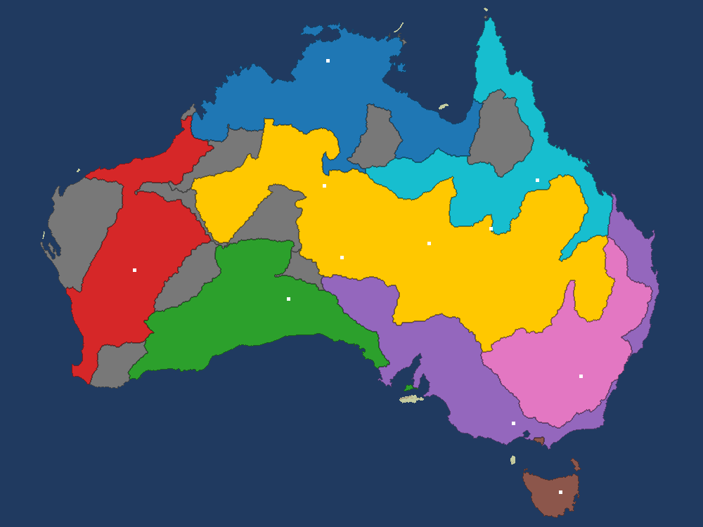
Minute 3, 37.8% of the land. The LLM (gold) spawned in the central
plains as the knowledge base advises, ate the tribes around it and allied with its
neighbours.
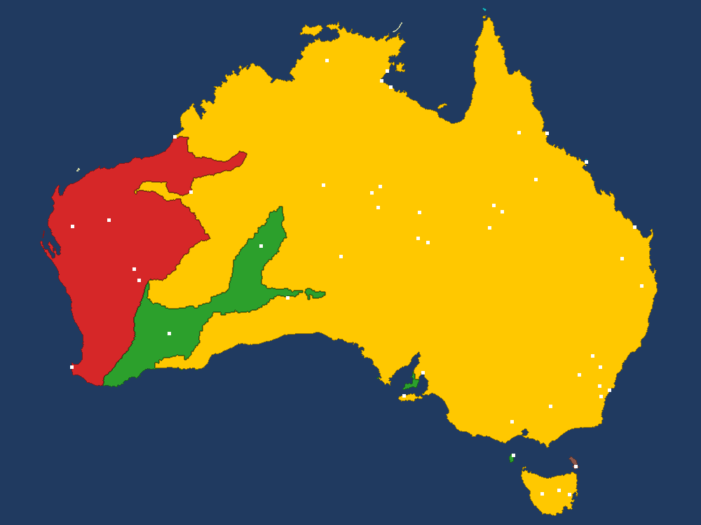
8:49, 80.9%, the game declares the LLM the winner. Once its
alliances expired, Victoria and New South Wales fell, then Queensland.
Iterating from the logs, on the same seed. Each failure was diagnosed by
reading turns.jsonl and fixed in the interface or the code.
Version
Setting
Result
Scripted players, no LLM
Medium
peak 5.8%, eliminated 6:21
Strategist + commander, the LLM controls every troop
Medium
peak 10.2%, eliminated 3:50
Same model, the code enforces reserve and waves
Medium, 3 min
24.1%, rank 1 of 11
Same agent, full game
Easy
won at 8:49, 80.9%
"Send troops to defend." The model kept attacking a stronger nation "to
defend", draining its army from 111,000 to 27,000. In OpenFront, troops kept at home
are the defence: a core rule now says so, and each attack option shows the
strength comparison next to its id.
Faster is not more reactive. A 1 s cadence repeated "expand 30%" and drained
the army in 10 s; a script with no LLM reproduced it. A troop budget per 5 s and a
reserve chosen by the plan took the same cadence from eliminated to first place.
Main takeaway: most of the improvement came from the interface (wording,
menu, schema, troop rules), not from the model.
Personal project. Multi-seed runs and ablations (knowledge base off, troop rules off) are the next
step. AGPL-3.0; independent of OpenFront.
The same few principles (a weighted sum, the chain rule, attention, a loss, a
feedback loop) are enough to go from the first artificial neuron to today's language-model
agents. This project proves it by building every step by hand, in 27
notebooks that each add one idea, implement it, check it against a reference library and
only then use the library. Everything runs on a MacBook Air M5, and every notebook is
saved with its outputs, so it can be read on GitHub without running anything.
1.93TinyStories loss of an 18M-parameter GPT trained in 14 min, against 2.63 for GPT-2
3.2 → 91.5%3-digit × 2-digit multiplication, same tiny Transformer, without and with a chain of thought
4 → 6 of 8bugs fixed by a coding agent once the harness runs the tests instead of trusting the model
01 — How it works
Build it, check it, then use the library
Backpropagation is derived by hand before an autograd engine is written; that engine
is checked against PyTorch before PyTorch is used. Attention comes before
nn.MultiheadAttention, a GPT before Hugging Face's, LoRA before
peft, PPO before any RL library, an agent loop before any framework and an
MCP server before the official SDK. Later modules import earlier ones: the coding agent
of module 24 runs on the agent loop of 22, which reuses the chat template of 19, which
fine-tunes the GPT of 14.
00 – 07
How networks learn
A numerical gradient checker, the perceptron and why XOR defeats it, softmax regression on MNIST in pure NumPy, a hand-derived MLP, a scalar then tensor autograd engine, optimisers from SGD to AdamW, and a small ResNet on CIFAR-10.
08 – 16
Language and Transformers
n-grams and perplexity, word2vec, LSTMs, attention, a BPE tokenizer compared with GPT-2's, a Transformer up to RoPE, a GPT that loads OpenAI's GPT-2 weights, a scaling sweep, a KV cache, mixture of experts, and a small ViT and CLIP.
17 – 21
Reinforcement learning and post-training
Q-learning, DQN, REINFORCE and PPO up to LunarLander; then GPT-2 fine-tuned into a chatbot (fully and with LoRA), a reward model, best-of-N and DPO, and GRPO with verifiable rewards on arithmetic.
22 – 26
Agents and the road to AGI
A tool-using agent loop with no framework, BM25 and embedding retrieval over the project's own notebooks, a coding agent and MCP from scratch, an evaluation harness, a sycophancy test, a sparse autoencoder, and measured open problems (continual learning, ARC).
02 — Skills
Deep-learning fundamentals. Backpropagation, initialisation, normalisation,
residual connections and optimisers implemented by hand and verified with a gradient
checker.
Transformers and LLMs. A GPT written from scratch that reproduces Hugging
Face's GPT-2 logits, plus scaling laws, mixed precision, a KV cache and
FlashAttention's online softmax.
Post-training. SFT, LoRA, reward models, DPO and GRPO, on models small enough
to train on a laptop.
Reinforcement learning. Value iteration, DQN, REINFORCE, GAE and PPO, with the
ablations that show why each ingredient is there.
LLM agents. Function calling, RAG, long-term memory, a coding agent and an
MCP client and server, on a 4B-parameter open model (Qwen3-4B).
Evaluation and interpretability. A benchmark harness with confidence intervals,
reward-hacking and sycophancy tests, and a sparse autoencoder on our own GPT.
03 — Results
Every number is measured in the notebooks, on a laptop. The notebooks also report
what did not work, and why: DQN without a target network, PPO without clipping, GRPO at
too high a learning rate, agents that claim fixes they never made.
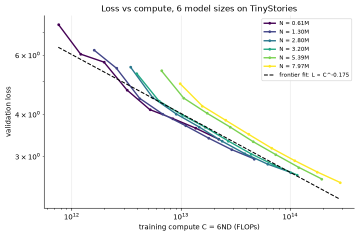
Module 15, a scaling law on a laptop. Six GPT sizes trained on
TinyStories; the compute-optimal frontier is a power law, L ∝ C−0.175, as in
Kaplan et al.
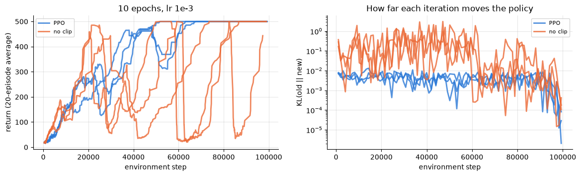
Module 18, why PPO clips. CartPole, 10 epochs per batch: without
clipping, each update moves the policy one to two orders of magnitude further and the
return collapses again and again.
Selected results. Each pair is the same model, with and without one idea.
Module
Without
With
19 · LoRA on 1.9% of the parameters
full fine-tuning, loss 2.077
loss 2.086
21 · Chain of thought, tiny Transformer
3.2%
91.5%
22 · Tools for a 4B model
1 of 8
7 of 8
23 · RAG over the project's notebooks
1 of 16
15 of 16
24 · Harness that runs the tests
4 of 8 bugs
6 of 8 bugs
PPO from scratch lands LunarLander in 96% of new episodes.
Interpretability. A sparse autoencoder finds a "dog" feature in our TinyStories
GPT; adding it while generating puts a dog in every story.
Main takeaway: on the agent side, every gain came from the loop around the same
model (tools, retrieval, a harness that checks), not from a bigger one.
Personal project. The models are scaled down to fit a laptop: a full
GPT-2 (124M) reproduction would take more than a month on it, as module 14 measures. MIT
licence; datasets and pretrained models keep their own licences.
Can an agent that learns by trial and error fly a fighter jet as well as a
hand-tuned autopilot? An agent trained on wrong physics learns to exploit the bugs, so
the project is split in two: jetfighter-sim,
an F-16 flight simulator written from the physics up and validated against published
data, and jetfighter-rl,
which turns it into a reinforcement-learning environment and trains agents on a
curriculum of manoeuvres, each judged against the classical autopilot.
01 — How it works
A curriculum, from easy to realistic
The agent first flies through the fly-by-wire (it commands g, roll rate and
throttle) on a fast simplified aircraft, then on the full rigid-body model, and
finally moves the control surfaces itself. Each task defines its own observations,
reward terms and success criterion.
Task
Success criterion
Recover wings-level from an unusual attitude
level within 10 s
Reach a heading, altitude and speed
within 30 m / 3° / 5 m/s, limited overshoot
Turn at the best sustainable rate
≥ 90% of optimal, no energy loss
Fly through 4 random 3D waypoints
all 4 captured
Loop, roll, Immelmann, Split-S
figure completed, right exit heading
02 — Skills
Reinforcement learning (RL). PPO (Stable-Baselines3, PyTorch) on a custom
Gymnasium environment, with curriculum learning and reward shaping from named,
separately logged terms.
Imitation learning. Behaviour cloning with DART noise and a critic
warm-up, needed where pure RL never finds a 20-second manoeuvre such as a loop.
Transfer learning. Policies trained on the simplified aircraft (3 DOF) are
copied into the full model (6 DOF) and fine-tuned (20% → 100% success).
Environment design. Observations without discontinuities (gravity
direction instead of Euler angles), a neutral action that holds the flight path, and
three clocks per step (100 Hz physics, 50 Hz fly-by-wire, 10 Hz agent).
Simulation and control. 6-DOF rigid body on NASA wind-tunnel data,
quaternions and RK4, gain-scheduled fly-by-wire, cascaded autopilot, LQR; 596
tests against analytic solutions and published F-16 figures.
03 — Results
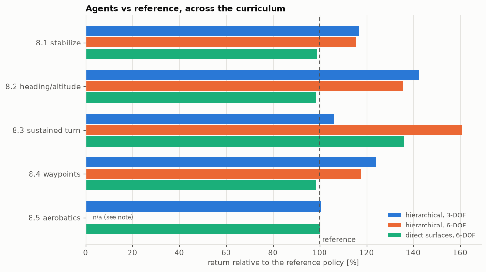
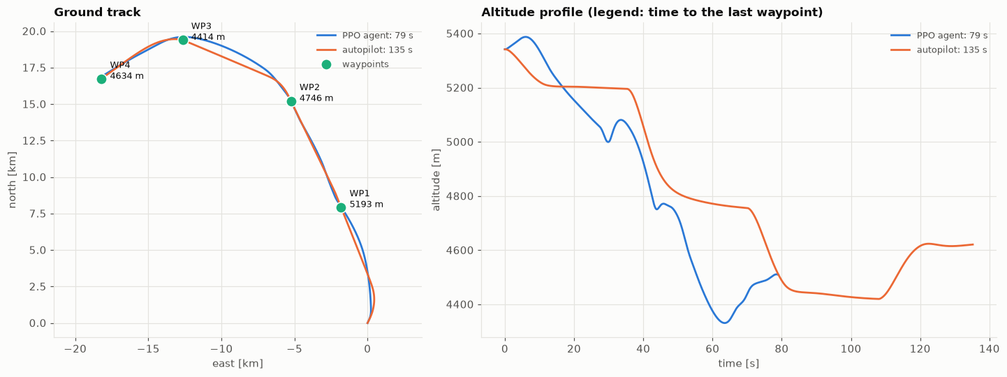
Through the fly-by-wire, agents match or beat the autopilot on all 5 tasks,
by up to 61% in return, with 90–100% success; a 4-waypoint course is flown in
79 s against 135 s.
Aerobatics learned by imitation then PPO: 100% success, slightly better
than the scripted pilot it learned from.
Without the fly-by-wire, moving the raw control surfaces: 90–100% success with
no envelope violation, at 72–84% of the fly-by-wire agents' return.
Return relative to the reference, one seed per agent. 100% means
matching the autopilot or scripted pilot on the same evaluation episodes. The 6-DOF
hierarchical aerobatics agent was trained before a reward hack was fixed and is left out.
Same course, same aircraft. The agent anticipates each turn and
trades altitude freely; the autopilot flies to one waypoint at a time.
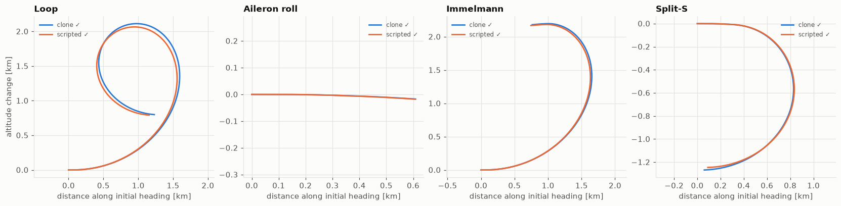
A network that was never rewarded, flying aerobatics. Loop, roll,
Immelmann and Split-S by the cloned policy against the scripted pilot it learned from.
Five reward hacks, none visible on the learning curves
Replaying the flights showed agents turning 2.5× faster than the optimum in a
descending spiral that lost 3 km, faking a loop with a 6-second wiggle, or crashing
early to stop paying costs. Each was closed by a reward fix, which is why the flights
were checked visually, not only on the metrics.
Personal project. Results are the best evaluated model of each
experiment on a single seed; more seeds are the obvious next step.
With a limited budget, where should cameras and radars go to protect a site? The
textbook answer maximises coverage. This project shows that coverage is the wrong
objective and replaces it, in three steps, with the question a security engineer
actually asks: will an intruder who knows the layout be detected in
time? Everything runs on a 3D model built from the Québec government's
airborne LiDAR (the site itself is fictitious).
Question
Metric
What it can hide
Is the site covered?
weighted coverage
the worst case
Will the intruder be detected?
detection on the least watched corridor
a blind corridor behind high coverage
Detected in time?
only detections earlier than the response
nothing: this is the design metric
01 — How it works
3D model
LiDAR tiles (30 points/m²) are streamed into terrain, building and canopy rasters. Buildings are opaque; trees are semi-transparent, with a transparency measured from the LiDAR itself.
visibility
An exact ray-tracing engine (numba) computes what each candidate position sees, then camera and radar detection laws give a detection matrix for 2,290 sensor configurations.
optimise
A greedy baseline, a MILP with cuts generated on demand that certifies how far from optimal each layout is, and NSGA-II for the cost / coverage / robustness trade-off.
adversary
An intruder finds the weakest corridor; each corridor becomes a new constraint for the optimiser, until no corridor remains and the layout is proven optimal.
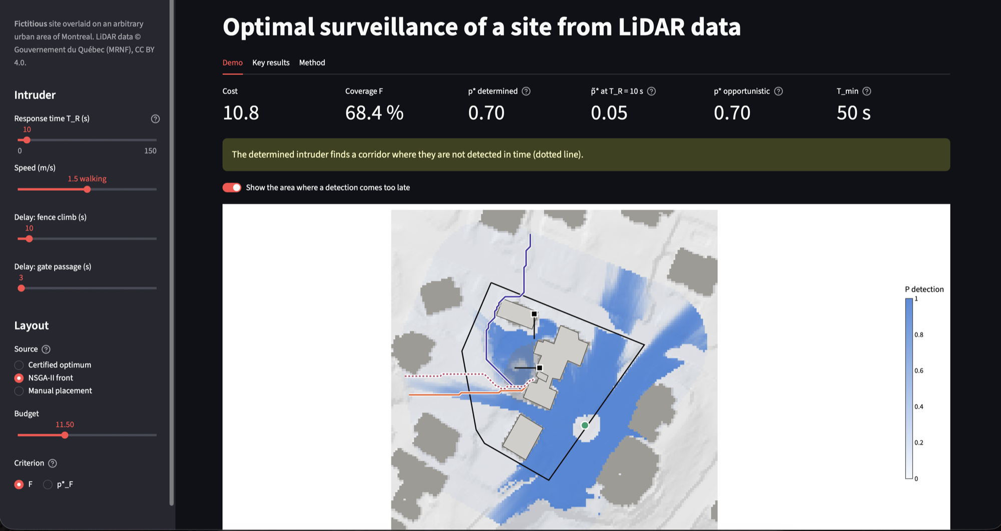
Three metrics, one layout, three verdicts. 68% coverage and 0.70 detection on the worst corridor, yet only 0.05 chance of detecting the intruder in time with a 10 s response.
02 — Skills
3D point-cloud processing. Classified LiDAR turned into terrain, building
and vegetation rasters at constant memory (PDAL, laspy, rasterio), checked against
PDAL and the official terrain model.
High-performance geometry. Exact ray traversal in a numba kernel, checked
against gdal_viewshed; an exact referee caught 1% of cells wrongly
marked visible by the first, sampled version.
Optimisation. Submodular coverage solved by greedy and by a MILP (HiGHS)
with lazily generated cuts, giving certified bounds; multi-objective search with
NSGA-II (pymoo).
Adversarial modelling. A worst-corridor metric computed exactly by
percolation (union-find), inside a master / oracle loop that converges with a
certificate.
Deep learning, used only where it is faster. A planned U-Net was
benchmarked and dropped where the exact engine was already faster; a PyTorch
surrogate was kept for whole-area visibility, with exact symmetry augmentation.
Decision analysis. Sensitivity measured as decision regret (summer
foliage, a running intruder), with the protocol fixed before computing anything.
03 — Results
The greedy heuristic loses up to 15.9 coverage points at one budget, a
loss that is visible only against the certified bound (optimum proven within 0.5% on
most budgets).
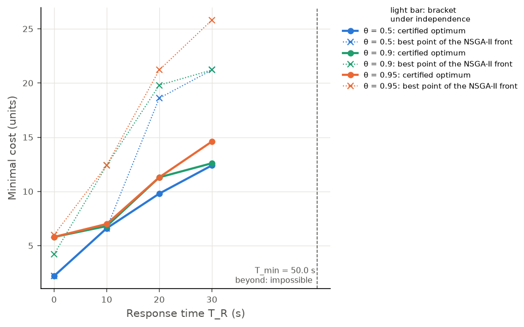
For a timely detection with a 10 s response, the certified layout costs
6.8 units against 12.4 for the best layout found by NSGA-II, which does not
optimise timing.
The fastest intrusion takes 50 s: with a slower response, no number of
sensors helps, only physical delay (fence, gates) does.
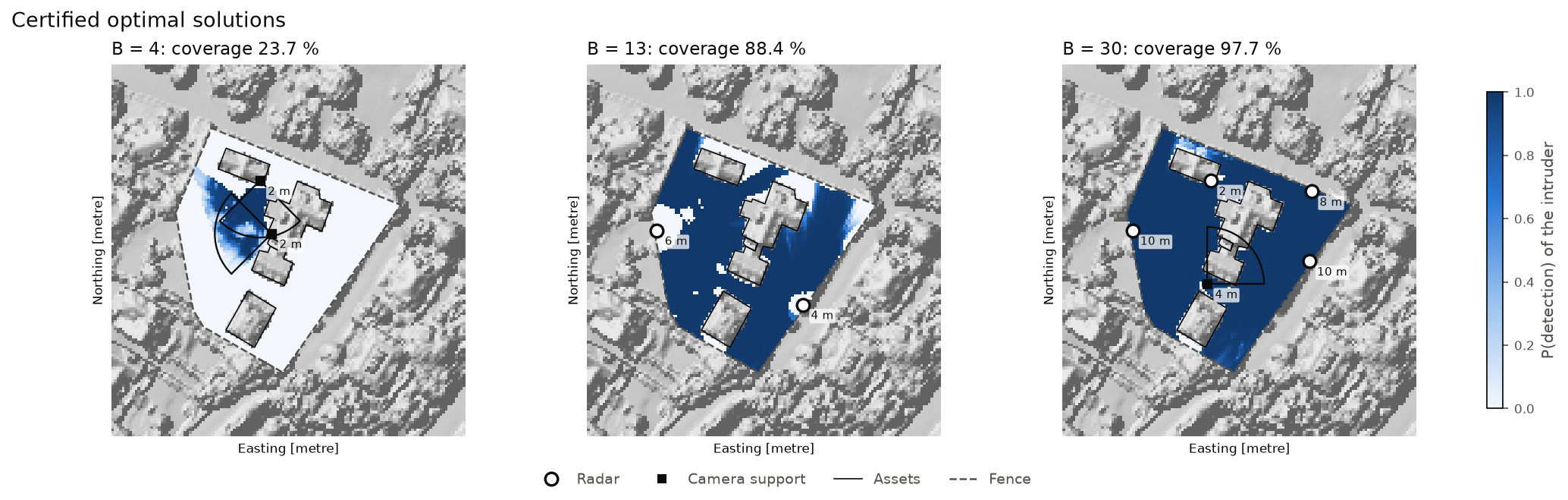
Certified optimal layouts. Cameras at small budgets, then radars, with a camera covering the radars' shadow.
The price of a timely detection. Certified optima (solid) against the best NSGA-II point meeting the same requirement (dotted).
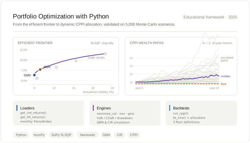
A series of 18 notebooks that builds a single Python risk toolkit, from measuring
returns to dynamic allocation. It starts with Markowitz optimisation and shows why it
is fragile, then moves to the question an investor with a future liability actually
faces: how to take market risk while guaranteeing a floor. Every
strategy is tested on 5,000 simulated scenarios and on 28 years of US market data.
0%floor breaches for the floor allocator, against 3.6% for 100% equities
−22%max drawdown of the constrained strategy, against −50% for the market, 1990–2018
0.55Sharpe ratio, against 0.46 for the market over the same period
01 — How it works
One allocation engine, several definitions of the floor
Strategies are written as allocator functions plugged into a backtester that knows
nothing about them. The core engine is CPPI: at each step, invest a multiple of the
cushion above the floor in the risky asset and the rest in the safe asset, so
exposure falls to zero before the floor is reached.
One engine, three definitions of the floor. The three dynamic functions share this exact loop and differ only in the line that updates F, which is what makes the jump from classic CPPI to liability-driven allocation nearly free.
02 — Skills
Numerical optimisation. Efficient frontier, max-Sharpe and minimum-variance
portfolios with SciPy SLSQP under constraints, and a demonstration of how a 1-point
error in expected returns sends the optimiser to a corner.
Monte Carlo and stochastic processes. Vectorised geometric Brownian
motion for equities and a CIR model for interest rates with analytic bond prices;
spotted a ~2% bias in a naive discretisation.
Risk measurement. Historic, Gaussian and Cornish-Fisher VaR, CVaR,
drawdown, skewness and kurtosis.
Backtesting design. Strategies judged on their full distribution
(probability and size of a shortfall), not on the average outcome.
03 — Results
The floor allocator eliminates every breach while giving up 0.03 of mean
terminal wealth; a 70/30 fixed mix gives up 0.21 and still breaches on 0.8% of
paths.
Raising leverage from 3 to 10 gains 0.02 of expected wealth and breaks the
guarantee on 2.8% of paths: gap risk.
On real data, the drawdown-constrained strategy halves the worst loss
and improves the Sharpe ratio, at a cost of 2.2 points of annual return.
5,000 scenarios, 10 years, binned terminal wealth. The fixed mix buys safety by cutting off both tails. The floor allocator does something else entirely: it stacks the failures into a spike just above 0.75 and leaves the right tail alone, its 95th percentile and its maximum are the same as pure equities'.
At a 3,000-guest student gala, bar stock was tracked with tally marks and guesswork.
This project aimed to design and deploy a connected system: an ESP32 button pad at every bar records
each sale, the data reaches a shared Google Sheet in real time over 4G, and a
lightweight forecast warns about 30 minutes before a bar runs out,
which is the time a runner needs to restock it.
01 — How it works
A button press is timestamped and queued on the device, then published over MQTT
through a private 4G router, independent of the venue's wifi. A bridge appends one row
per sale to the Google Sheet, removing duplicates by sequence number, and the
forecast reads the same sheet.
One loop, closed at the storeroom. The left column is the only part
that lives in the venue; everything to the right of the 4G uplink is off site, which is
what makes the sheet survive a bar losing power or a device being unplugged mid-evening.
02 — Skills
Embedded and IoT. ESP32 firmware in C++, a button matrix, and a local
queue so the bartender never waits for the network.
Reliable messaging. MQTT over 4G with sequence numbers, so a device can
resend freely after a reconnection without inflating sales.
Real-time forecasting. Last year's consumption profile, adjusted for the
moment of the night and the bar's location, re-anchored on live sales; the alert
fires when the projected time to empty reaches the restocking time.
User-centred design. A Google Sheet as the dashboard, because the whole
team already had it on their phones.
03 — Results
Used for one night across several bars and 3,000 guests, with stock-out warnings
about 30 minutes ahead. The night ends with a per-second record of what was sold
where, which is what next year's forecast is fitted on.
One bar, one night, reconstructed for this page. The dashed curve is
the prior, the solid one is what the presses actually say, and the alert is not raised
when the stock is low but when the projected time to empty falls to the runner's round
trip.
Built for a student gala, 2023. The firmware, bridge and forecasting
sheet were written for the event and are not public; figures are redrawn from the
evening's logs.
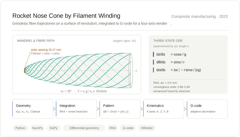
A semester project for the CNES PERSEUS programme at Arts et Métiers: a rocket nose
cone wound from flax fibre on a four-axis winding machine. A fibre laid along the wrong
path slides down the cone before the resin cures, which is what the first trials
showed. My part was the mathematical and software chain: model the fibre path,
simulate the whole winding and generate the machine program.
3.99measured convergence order of the RK4 solver (4 expected)
26.2708 mmpolar opening found by the solver, against 26.271 mm in closed form
×9.710,597 path points compressed to 1,095 G-code blocks within 0.05 mm
01 — How it works
The fibre path is the solution of a three-equation ODE built from the surface
geometry and one friction parameter. Everything downstream (pattern, coverage,
machine axes, timing, G-code) is computed from that one trajectory.
One model, two consumers. Everything above the fold is geometry and
the ODE; everything below it is bookkeeping on the solution. The coverage branch and
the machine branch read the same trajectory, which is why a coverage requirement can be
turned directly into a pattern and a cycle time.
02 — Skills
Mathematical modelling. Differential geometry of the mandrel and a
no-slip criterion that says when friction can hold a fibre in place.
Scientific computing. RK4 integration in arc length, which removes the
singularity of the textbook formulation at the turnaround; turnarounds located by
bisection; a conserved quantity used as a free error check.
Algorithm design. The pattern algebra that explains why one extra circuit
can nearly double the fibre used, and a G-code compression by exponential and binary
search.
Robotics and CNC. Four-axis inverse kinematics, speed planning within the
axis limits, and G-code generation for the real machine.
03 — Results
Explained the slippage and fibre build-up seen in the trials: at the small end,
the path required more friction than was available.
A design recipe for a closed layer, 30 circuits with pattern number 7,
predicted from the algebra, then confirmed by a simulation it had never seen
(coverage 1.016 for a target of 1).
A machine program that accounts for the offset of the fibre-delivery eye, which
would otherwise misplace the spindle by up to 20.9°.
The bare mandrel. The turned nose cone profile, mounted between
chucks on the XWinder before any fibre is laid.
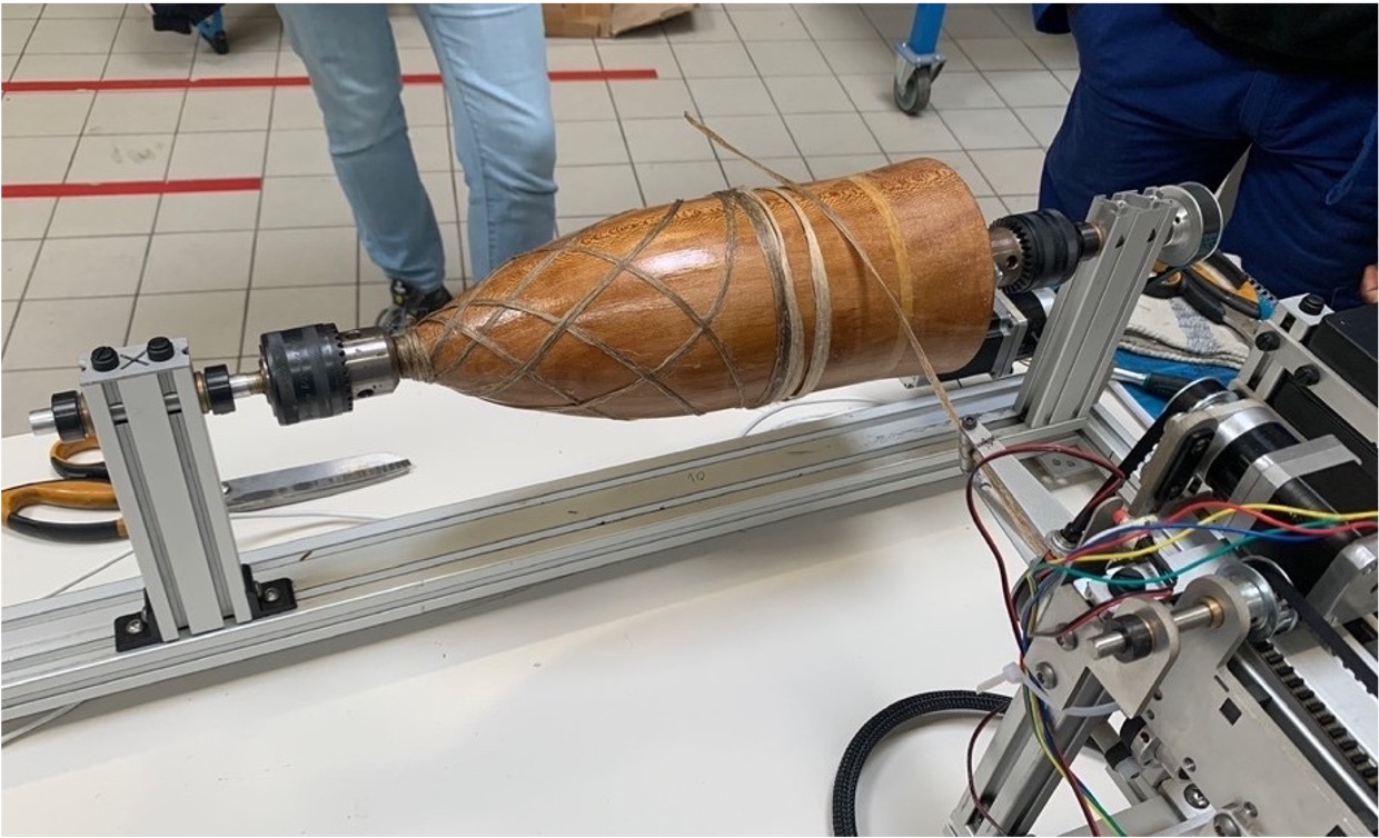
After a few passes. The crossings of the flax tow are the band
pattern the algebra of section 09 predicts, laid on the real surface.
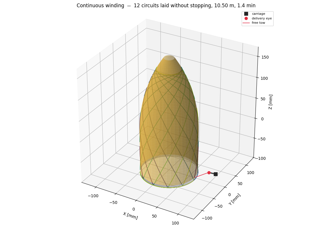
Twelve circuits, laid without stopping. 10.50 m of tow in 1.4 min.
The carriage, the delivery eye and the free length of tow between them are simulated
with the path, since the eye lead is what the inverse kinematics has to solve for.
Semester project for the CNES/PERSEUS programme, ASTREOS demonstrator,
at Arts et Métiers. The project report also covers the flax/Elium materials, the machine
and the experimental campaign; this page covers the mathematical and software parts.